Frog A & B

Frog A
Solution to Frog A:

1. There's only 1 state, which is the stone number on which the frog is on. The subproblem can be framed as the min cost to reach i^th stone. In terms of implementation, Dp[i] is the min cost for frog to reach the ith stone from 1st stone.
2. Base case: dp[0] = 0, because the cost of reaching to the current stone is zero
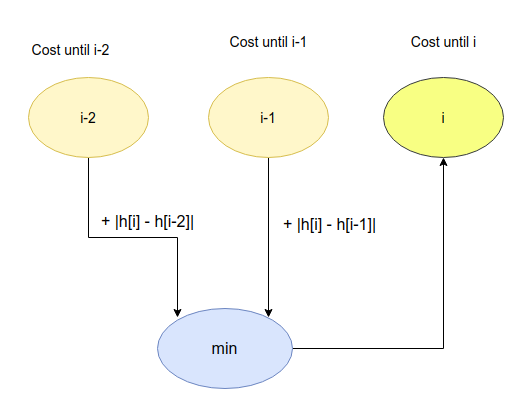
3. Transitions: Frog on ith stone can either be reached from i-1th stone, or i-2th stone. According to the problem, Cost of hopping from xth stone to yth stone is |h[x] - h[y]|.
   In order words, dp[i] = min(dp[i-1]+|h[i]-h[i-1]|), dp[i-2] + |h[i]-h[i-2]|)

Now since we have defined the states,base cases and transitions, let us look at the code for frog A

Frog B
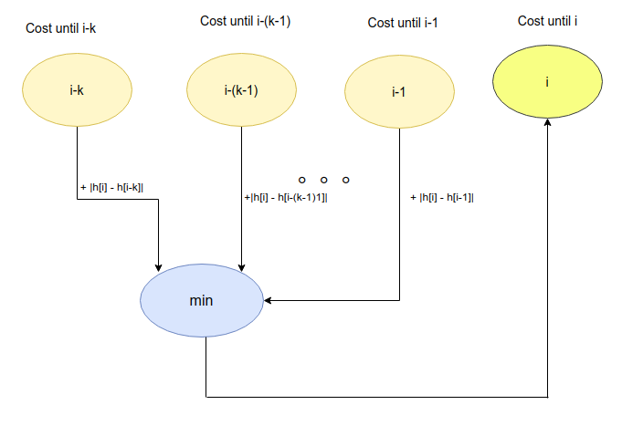
Frog B is extremely similar to frog A, except for the fact that we will be dealing with upto n transitions.
In other words, dp[i] = min(dp[i], dp[i-1] + |h[i]-h[i-1]|, dp[i-2] + |h[i] - h[i-2]|, ... , dp[i-k] + |h[i] - h[i-k]|)

Here's the code for the code for the same:

AtCoder Vacation

Frog B

The problem asks you to find the max 'fun' given that no same activity can be done in 2 consecutive days.

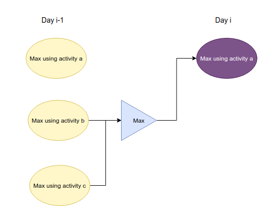
Intuition: If activity a is done on day i, then activity that can be done on day i-1 can either be activity b or c.

1. Using the intuition, we can define the state of the dp as: dp[i][j] be the max fun given that activity i is done at day j
2. Dp array structure: dp[number of activies][days]. In other words, here it is a 3*n array
3. Base cases: dp[0][0] = activity_a[0], dp[1][0] = activity_b[0], dp[2][0] = activity_c[0]
4. Transitions: In English: max possible value of activities other than the current activity until yesterday + today's activity.
   Mathematically,
   dp[0][i] = max(dp[1][i-1],dp[2][i-1]) + activity_a[i],
   dp[1][i] = max(dp[0][i-1], dp[2][i-1]) + activity_b[i],
   dp[2][i] = max(dp[0][i-1], dp[1][i-1]) + activity_c[i]
   Below is transition diagram for the 1st recurrence relation. Code for the same:
   

Knapsack 1

KnapSack 1

This problem is the classical 0/1 Knapsack problem. Given a set of n items each with weight w[i] and value v[i], and a sack which can hold atmost weight of W, find the maximum value you can hold using the sack.

Approach: There are 2 parameters that are crucial in determining the problem's outcome.

1. The index upto which the items are being considered
2. The capacity of the knapsack

These 2 are the states in this problem. More specifically, dp[i][j] represents the max value obtainable considering items upto index i, with capacity j. If you're having trouble coming up with the states, try writing the recursive code for knapsack first. The parameters that guide the recursion are the states. The recursive code looks something like this:
# i: current index, C: capacity
# call: f(N,W)
f(i,C,w[],v[]):
  if i < 0:
    return 0
  if w[i] > C:
    return f(i-1,C,w,v)
  return max(f(i-1,C,w,v), f(i-1,C-w[i],w,v) + v[i])

Base cases: For weight 0, all entries will be zero
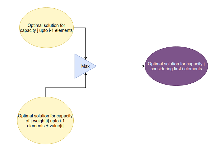
Transitions: To reach the current state dp[i][j], it could
either pick the current item and use the remaining capacity optimally, or
skip the current item and use the remaining capacity optimally
Mathematical recurrence for the same is: dp[i][j] = max(dp[i-1][j-w[i]] + v[i], dp[i-1][j])
Transition diagram:
Note: Handle the case where the current element is greater than capacity by an if-else.
Code:

AtCoder E: Knapsack 2

KnapSack 2

This is a variant to the knapsack, where the constraints on weights are larger ~(10⁹). So, our previous solution, which uses weight as one the states will make the problem computationally infeasible. However, take note of the constraints of values. No value is greater than 10⁵, and the maximum number of items is 100. In other words, the sum of all values cannot be larger than 10⁷. Now the problem reduces to reframing the question, to use the 'value' state: (ranges from 0 to sum of all values).

We reframe the question as follows: Given a particular value, what is the minimum possible weight usable to get this value? (Return infinity if it is not possible to reach the value). Then, we can iterate over the range of reachable values(0 to sum(val)) and get the largest value for which the answer(i.e the min weight) is <= knapsack's cap.
Let us look at the states,base case, and transitions for this problem.

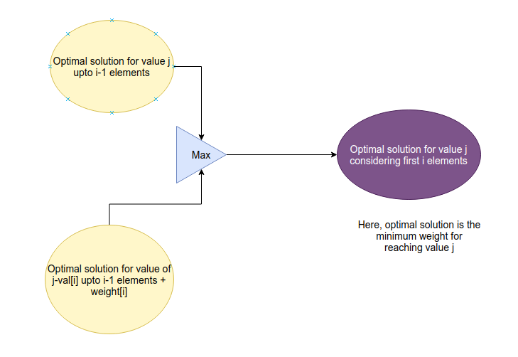
1. State: dp[i][j] represents the minimum possible weight by using the first i items to get value j. Array will be: dp[n][sum of values]
2. Base case: dp[0][0] = 0, dp[0][v[0]] = w[0]
3. Transition: Current state dp[i][j] can either be having the optimal solution by either
   Ignoring the current item and using the optimal solution defined for i-1 items or
   Using the current item and optimal solution defined for leftover values for i-1 items
   Transition rule: dp[i][j] = min(dp[i-1][j], dp[i][j-v[i]] + w[i])
   Note: During implementation handle the case where j < v[i]
4. Finally iterate over the last row (the solutions that include all elements) the find the max value for which the minimum possible weight is <= knapsack cap.

Implementation:

Longest Common Subsequence (LCS)

LCS

Classic LCS: Given strings s and t, find out (any one) longest common subsequence. Our strategy will be to first build the table for the finding optimal length of lcs, and then using the table to pick the lcs.

1. The states in this problem are the lengths upto which we are considering the strings. Specifically, dp[i][j] represents the length of longest subsequence when considering first i characters of string s and first j characters of string t.
2. Dp table will be of form dp[len(s)+1][len(t)+1]
3. Base case: dp[0][0] = 0
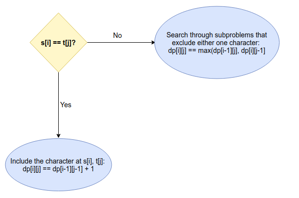
4. Transition: Considering the lcs of strings s,t upto length i and j respectively. Now,
   Either s[i] == t[j], in which case the optimal solution would be dp[i-1][j-1] + 1. (Including both of the last characters from strings is better skipping one)
   Otherwise, the characters do not match, in which case we look for the optimal solution by searching in the subproblems that consider i-1,j and i,j-1 states.
   Transition rule:
   if s[i-1] == t[j-1]: #0 based indexing, hence then -1
   dp[i][j] = dp[i-1][j-1] + 1
else:
   dp[i][j] = max(dp[i-1][j],dp[i][j-1])
   
5. Finally, we use the dp table to traverse accross the strings (in reverse) in an optimal manner to build the lcs. When there is a match, add the character. Otherwise decrement the pointer of the string whose subproblem's answer is greater.

Here's the implementation of the same:

Longest Path

Longest Path

Given a Directed Acyclic Graph, find the length of the longest path.

This problem requires the second style of dynammic programming, memoization. We write a recursive code and memoize it using a single state dp array, which remembers the solutions to the subproblems, so that they are not recomputed. The main idea is to use dfs on all vertices seperately, and return the max length of the path which starts from that vertex.

Note: One vertex might be involved in multiple paths, therefore it is not possible to arrive at a correct answer by just visiting the vertex once.
This problem doesnt really require transition rules or diagrams, as it is simply a memoization over the classic recursive dfs.
Below the implementation for the same:

Grid 1

Grid 1

Given a grid with connectable rooms and blocked rooms, find the number of ways to reach the destination h,w from start 1,1.

1. States: i,j: i for rows, j for columns. dp[i][j] represents the number of ways to reach point i,j from 1,1
2. Base cases: The first row and first column will be intialized with 1s, until there is a blocked room. Upon meeting a blocked room, the subsequent entries the row/column will all be 0.
3. Transition: You can only move right or down, so a state can only be reached from preceeding left or up states. Also, it is never possible to reach a blocked room.
   Transition rule:
   if grid[i][j] is a connecting room:
   dp[i][j] = (dp[i][j-1] + dp[i-1][j])


Here's the implementation for the same:

Coins

Coins

Given N coins and the probabilities of getting heads for each coins respectively, find the probability of getting more heads than tails. This is a nice introduction to probability dp problems. It's not really that different from a classic dp problem.

1. States: i the number of tosses done, j number of heads. dp[i][j] Probability of getting j heads in i tosses.Dp table: dp[n][n+1]
2. Base case: dp[0][0]: 1 - p[0](Tails on toss 1), dp[0][1] = p[0](Heads on toss 1).
3. Transition: 2 possiblities:
   Heads on ith toss: -> Probability of heads on ith toss, then you multiply that with probability of getting j-1 heads upto i-1 tosses
   Tails on ith toss: -> Probability of tails on ith toss, multipied by the probability of getting j heads upto i-1 tosses.
   

Code:

Final Problem: Sushi

Sushi

This is difficult problem. The problem states that you are given n plates, where each plate is one of the 4 types of plates of sushis, plates with 3,2,1 and 0 sushis. You have to calculate the expected number of operations till all the plates are empty.

Observation 1: The plates belonging to the same category are identical. This means that order does not matter. We only need to concerned with the counts of 3-plates,2-plates,1-plates, and 0-plates.

Observation 2: sum of all types of plates = n. Therefore we can rewrite 0-plates as: n - (3plates+ 2plates + 1plates), and avoid storing 0 plates as a seperate state.

1. From Observation 1 and 2, we can see that the states needed are: 3-plates, 2-plates and 1 plates. dp[i][j][k] represents the expected number of moves for i 3-plates, j 2-plates and k 1-plates.
2. Base case: dp[0][0][0] = 0
3. Transitions:
   Case 1: 3-plate is picked. 1 sushi is eaten, the number of 3-plates reduce by 1, and the number of 2-plates increases by 1. This contributes to the term p3 * dp[i-1][j+1][k] , where p3 is the probability of picking a 3-plate.
   
   Case 2: 2-plate is picked. 1 sushi is eaten, the number of 2-plates reduce by 1, and the number of 1-plates increases by 1. This contributes to the term p2 * dp[i][j-1][k+1], where p2 is the probability of picking a 2-plate.
   
   Case 3: 1-plate is picked. 1 sushi is eaten, the number of 1-plates reduce by 1, and the number of 0-plates increases by 1. This contributes to the term p1 * dp[i][j][k-1], where p1 is the probability of picking a 1-plate.
   
   Case 4: 0-plate is picked. No sushi is eaten, This contributes to the term p0 * dp[i][j][k], where p0 is the probability of picking a 0-plate. Because dp[i][j][k] is unknown, we can transpose this term to the LHS to work around this. Detailed explanation is in the code.
   
   * Always add 1, because no matter what the choice, one move is going to be made.
4. Invalid state elimation: During a loop, if i+j+k > n, it is invalid, because the no valid state will have more than n plates. Further, if i+j+k = 0, it is a trivial state and can be skipped.
5. Ordering: Looking at the transitions, 3-plates state is dependent on 2-plates state, 2-plates-state is dependent on 1-plate state. Therefore, subproblems should be ordered such that the 1-plates should be calculated first, followed by 2 plate-states, followed by 1-plate state.

Below is the implementation:

Concluding Remarks: General approach to DP Problems

In this article we talked about what dp is, the necessary theory behind it, followed by solving standard dp problems. At the end, I'd like to once again, emphasize the way of thinking in dp problems. To break it down, the flow goes like:

• Identify the problem is dp
• Come up with states and define the subproblems
• Come up with the transitions between the states and formulate the transition rules
• Observe the base cases and necessary constraints
• Implement

This requires some practice to get used to, but after solving a few problems, the whole process starts seeming more natural.

Well then, until next time!